
The algorithm for linear asset inspections
This algorithm has been designed to optimize the ordering of inspection tasks on linear assets, such as power lines. The goal is to create a logical and efficient sequence for field technicians to follow, minimizing travel and wasted time.
How the algorithm works
The algorithm:
-
Reconstructs the structure: The algorithm first reconstructs the linear asset's structure based on the geographic coordinates of its segments and points. Two points are considered connected if the distance between their endpoints is within a specified, configurable threshold.
-
Determines the sequence: The sequence of operations is determined by following the linear continuity of the segments.
-
Selects the next segment: If there are multiple segments, the algorithm chooses the next one based on proximity to the current end point. It selects the segment with the closest starting or ending point.
To calculate an efficient linear sequence for field technicians’ inspection tasks, the algorithm:
-
Reconstructs the linear asset’s structure to connect coordinates of its segments and points within a specified, configurable threshold.
-
Determines the sequence by following a continuous line of the segments.
-
Selects the next segment closest to the current end point.
Understand the algorithm for linear asset inspections
To calculate an efficient linear sequence for field technicians’ inspection tasks, the algorithm:
-
Reconstructs the linear asset’s structure to connect coordinates of its segments and points within a specified, configurable threshold.
-
Determines the sequence by following a continuous line of the segments.
-
Selects the next segment closest to the current end point.
Example
Below is an example showing a linear asset with four segments: A, B, C, and D.
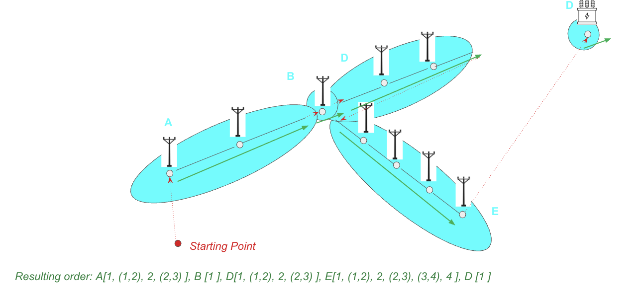
To order the inspections in this example, the algorithm:
-
Creates a starting point: The process begins at a designated starting point, which can be an operation within the bundle itself. In the example, let's assume the starting point is in a geographical point close to the beginning of segment A.
-
Navigates the first segment: First, the algorithm orders the inspections on segment A, following its linear continuity. This results in an order like:
A[1, (1,2), 2, (2,3)].
-
Chooses the next segment: From the end of segment A, the algorithm decides which segment to visit next. It evaluates the segments that are connected (or close enough based on the configurable threshold). In the diagram, segments B and D appear to be the closest. The algorithm would choose the one with the closest starting or ending point. In this case, let's say it's segment B.
-
Navigates the next segments: After visiting segment B, the algorithm would then choose the next closest segment, which might be D , and so on, creating an efficient, continuous route.
This logic can be extended to include other criteria, such as selecting the next segment based on shortest duration or the highest number of operations. This ensures that the route is not just continuous but also optimized for efficiency.